
Brandon Sepulvado


In my first post, I am going to begin what will most likely be a three-part series on the evolution of bioethics publications over the last several decades. This post is mostly about getting the data in order and exploring what the amazing tidytext package has to offer.
Bioethics has emerged over the last several decades from several branches of ethics (e.g., medical and religious) to form a domain with its own set of conceptual and institutional structures. In this series of posts (and the associated paper), I examine the conceptual structure of bioethics in the English-speaking world.
The data I use come from the Web of Science (WoS). On 12 January 2018, I downloaded all records of all types of texts (e.g., journal articles, books) written between 1900 and 2018 in English, as indicated by the title (TI) or subject (TS) fields, containing the stem “bioethic”; records came from the WoS Core COllection: SCI Expanded, SSCI, A&HCI, CPCI-S, CPCI-SSH, and ESCI. 8,150 records met these criteria. Unfortunately, given the licensing requirements, I cannot make the data available.
First, the necessary packages need to be loaded. I will load, at a later point, some other packages, but certain important functions will be masked. Thus, I will wait to load them.
library(tidytext)
library(readxl)
library(dplyr)
library(stringr)
library(ggplot2)
library(tidyr)
library(igraph)Because the records I will analyze are fairly circumscribed (n = 8,150), I did not use the API to download a single data file; rather, I used the GUI within the WoS to download the information. As a result, I could only download 500 records at a time, which gave me a series of several files needing to be merged.
I used a standardized naming convention when downloading the files, so the first thing I do is create a list of file names that will be used to load the individual data files into another list. For this section, I used .xlsx files on tab separated filed provided by the WoS.
Step one: create a vector a record ranges.
ranges <- c("1-499", "500-999", "1000-1499", "1500-1999", "2000-2499", "2500-2999", "3000-3499", "3500-3999", "4000-4499", "4500-4999", "5000-5499", "5500-5999", "6000-6499", "6500-6999", "7000-7499", "7500-7999", "8000-8150")Step 2: create a vector for file names.
files <- vector(mode = "character", length = length(ranges))Step 3: populate the files vector (not shown).
Everything looks on track at this point. However, before importing these files into R, I first want to create an empty list for which each of the corresponding .xlsx files will constitute a member.
bioeth.data <- vector("list", length(files))This code creates the bioeth.data list, which has the same length as the files vector. Running the following, we see that everything looks good.
glimpse(bioeth.data )## List of 17
## $ : NULL
## $ : NULL
## $ : NULL
## $ : NULL
## $ : NULL
## $ : NULL
## $ : NULL
## $ : NULL
## $ : NULL
## $ : NULL
## $ : NULL
## $ : NULL
## $ : NULL
## $ : NULL
## $ : NULL
## $ : NULL
## $ : NULLWe can see that the code created a list of 17 elements, currently having no contents.
Now, we can import each file into a list element. Several warnings will show up because R is expecting a numeric format for certain rows and receives a date; these warnings will not affect later results.
for (j in 1:length(files)) {
  bioeth.data[[j]] <- read_excel(files[j])
}
Before merging the list members together (i.e., the different sections—of rows—of the data set that will ultimately exist), I will remove the columns in which I am not interested; this task simply involves telling dplyr to select the columns of interest.
for (i in 1:length(bioeth.data)) {
  bioeth.data[[i]] <- select(bioeth.data[[i]], PT, AU,
                             AF, TI, SO, DT, DE, ID, AB,
                             C1, CR, TC, Z9, PU, PD, PY,
                             DI, D2, WC, SC)
}
Finally, the moment has arrived: collapsing the list into a single data set.
data.bioeth <- bind_rows(bioeth.data)To check that this went correctly we can use class(data.bioeth) and dim(data.bioeth) to verify the class and dimensions of this new data set. We should see that the structure is a tibble because we are relying on packages from the tidyverse and that the number of rows is equal to 8,150, the number of records downloaded from the WoS. We have 20 variables.
## [1] "tbl_df" "tbl" "data.frame"## [1] 8150 20The data.bioeth object thus has the desired class and dimensions, yet, checking names(data.bioeth), the column names are still the two letter identifiers from the WoS. Let’s change them to more intuitive names.
data.bioeth <- rename(data.bioeth,
                      pub.type = PT,
                      authors = AU,
                      author.full = AF,
                      doc.title = TI,
                      pub.name = SO,
                      doc.type = DT,
                      author.keywords = DE,
                      keywords.plus = ID,
                      abstract = AB,
                      author.address = C1,
                      cited.refs = CR,
                      wos.core.citedcount = TC,
                      total.cited.count = Z9,
                      publisher = PU,
                      pub.date = PD,
                      year.pub = PY,
                      doi = DI,
                      book.doi = D2,
                      wos.categs = WC,
                      research.areas = SC)
With the rename function of the dplyr package, the new variable names go first.
Now that the data have been imported, I will look at the use of single keywords. Before getting going any further, I want to add a unique numerical identifer for each record. The WoS provides multiple options, such as the DOI, but even these have missing data.
data.bioeth.1 <- data.bioeth %>%
  mutate(article.id = seq(from = 1, to = nrow(data.bioeth), by = 1))
The goal of this section is to examine keywords provided by the author (author.keywords), which are currently stored in a single cell. In addition, I want to remove stop words and records for which no keywords were provided (NA). However, the words would still be stored within a single cell.
The unnest command from the tidytext package helps. From each cell, it removes punctuation, restructures the data such that a single keyword populates a single keyword cell, and transfers any other information on the record to the new rows. Basically, whereas previously each record had one row, a WoS record now has as many rows as it has keywords. The filter command removes NAs, and the anti_join command removes stop words; in the latter, we must specify from which column to remove the stop words. (If the column of keywords were named “word”, this extra step would be unnecessary.)
data("stop_words")
unnest.akw <- data.bioeth.1 %>%
  filter(!is.na(author.keywords)) %>%
  unnest_tokens(akw, author.keywords) %>%
anti_join(stop_words, by = c("akw" = "word")) Now, let’s look at the 10 most commonly used words.
unnest.akw %>%
  count(akw, sort = TRUE) %>%
  head(10)
## # A tibble: 10 x 2
## akw n
## <chr> <int>
## 1 bioethics 2205
## 2 ethics 1699
## 3 research 763
## 4 health 593
## 5 medical 440
## 6 care 411
## 7 human 393
## 8 consent 332
## 9 life 265
## 10 informed 264The first two words are used drastically more often than the others, and, given that they are bioethics and ethics,it should be no surprise. Let’s remove them and reexamine the most commonly used words.
unnest.akw %>%
  filter(akw != "bioethics" & akw != "ethics") %>%
  count(akw, sort = TRUE) %>%
  head(10)
## # A tibble: 10 x 2
## akw n
## <chr> <int>
## 1 research 763
## 2 health 593
## 3 medical 440
## 4 care 411
## 5 human 393
## 6 consent 332
## 7 life 265
## 8 informed 264
## 9 clinical 260
## 10 autonomy 228Now, let’s look at the journals. The following code shows the number of different publication types present in the data set and how many distinct journals are cited.
unnest.akw %>%
  summarise(n_distinct(pub.type), n_distinct(pub.name))
## # A tibble: 1 x 2
## `n_distinct(pub.type)` `n_distinct(pub.name)`
## <int> <int>
## 1 3 1148unnest.akw %>%
filter(pub.type == "J") %>%
summarise(n_distinct(pub.name))## # A tibble: 1 x 1
## `n_distinct(pub.name)`
## <int>
## 1 1027That is a lot of journals. I assume that there is a gross inequality in the number times these journals appear in the data, but, to be sure, I am going to plot the distribution of the number of times journals appear in the data.
unnest.akw %>%
  filter(pub.type == "J") %>%
  count(pub.name, sort = TRUE)
## # A tibble: 1,027 x 2
## pub.name n
## <chr> <int>
## 1 JOURNAL OF MEDICINE AND PHILOSOPHY 1562
## 2 BIOETHICS 1544
## 3 THEORETICAL MEDICINE AND BIOETHICS 1078
## 4 JOURNAL OF BIOETHICAL INQUIRY 1049
## 5 DEVELOPING WORLD BIOETHICS 948
## 6 MEDICINE HEALTH CARE AND PHILOSOPHY 906
## 7 SOCIAL SCIENCE & MEDICINE 880
## 8 CHRISTIAN BIOETHICS 754
## 9 AMERICAN JOURNAL OF BIOETHICS 684
## 10 HEALTH CARE ANALYSIS 538
## # ... with 1,017 more rowsunnest.akw %>%
filter(pub.type == "J") %>%
count(pub.name, sort = TRUE) %>%
ggplot(aes(n)) +
geom_histogram(show.legend = FALSE) +
xlab("Number of times cited") +
ylab("Count") +
ggtitle("Histogram of journal citation counts")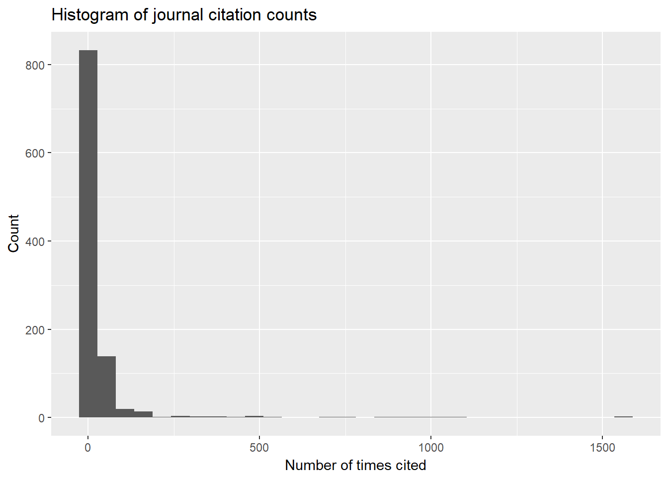
unnest.akw %>%
  filter(pub.type == "J") %>%
  count(pub.name, sort = TRUE) %>%
  ggplot(aes(n)) +
  geom_histogram(show.legend = FALSE) +
  xlim(0, 250) +
  xlab("Number of times cited") +
  ylab("Count") +
  ggtitle("Histogram of journal citation counts, adjusted x-axis")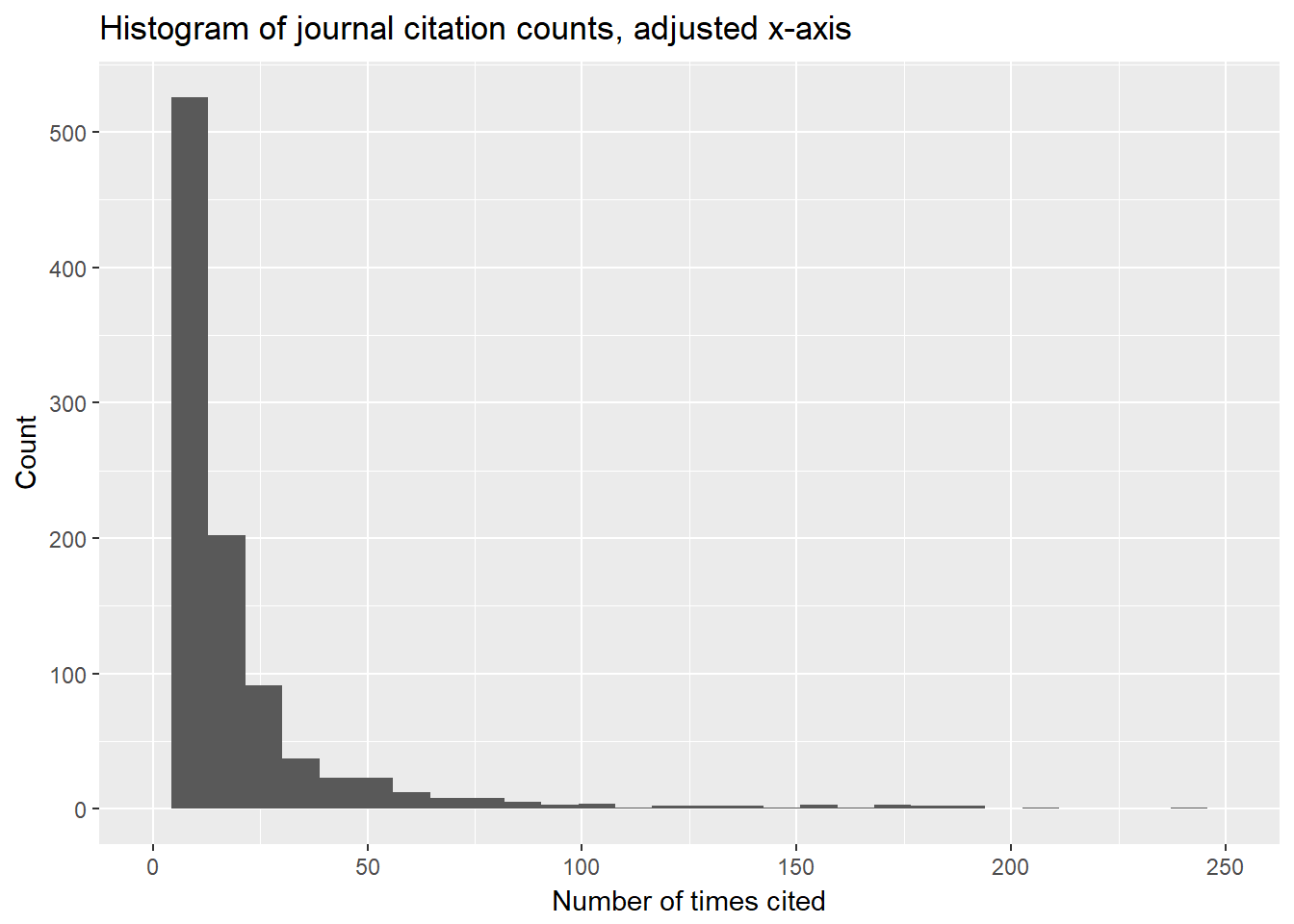
To summarize before going further, the goal is to get a data object for which a row is a unique “keyword + article” unit. We currently have this structure, but, given the above results, I want to remove “ethics”, “bioethics”, and keywords containing numbers. Thus, I will here create a final version of the unnest.akw object.
akw.art.final <- data.bioeth.1 %>%
  filter(!is.na(author.keywords)) %>%
  unnest_tokens(akw, author.keywords) %>%
  anti_join(stop_words,
            by = c("akw" = "word")) %>%
  filter(akw != "bioethics" &
           akw != "ethics") %>%
filter(!str_detect(akw, "\\d"))I now want to turn to examining which words are most representative of certain journals and which provide little distinction. Thus, I turn to the tf-idf. Yet, before going any further, I want to create a new object based on the filtering I did a few steps ago; that is, I want to select only those article appearing in journals.
# with years column
akw.j.noyears.final <- akw.art.final %>%
  filter(pub.type=="J") %>%
  select(akw, pub.name) %>%
  rename(keyword = akw, journal = pub.name) %>%
  count(keyword, journal, sort = TRUE)

# no years column
akw.j.years.final <- akw.art.final %>%
  filter(pub.type=="J") %>%
  select(akw, pub.name, year.pub) %>%
  rename(keyword = akw,
         journal = pub.name,
         year = year.pub) %>%
  count(keyword, journal, year, sort = TRUE)
These two objects also contain n, a column indicating how frequently each author keyword (akw) occurs within each journal.
To calculate the tf_idf, I need the weighted edge list, in which keywords are linked to the journals in which they appear, as well as the total number of times keywords appear in a given journal. The akw.j.noyears.final is essentially a weighted edge list between keywords and journals, and total.words contains the total number of keyword occurences in a journal. The tidytext package makes calculating the tf_idf quite easy.
total.words <- akw.j.noyears.final %>%
  group_by(journal) %>%
  summarize(total = sum(n))

journal.words <- left_join(akw.j.noyears.final,
                           total.words)
## Joining, by = "journal"journal.words <- journal.words %>%
bind_tf_idf(keyword, journal, n)
journal.words## # A tibble: 21,042 x 7
## keyword journal n total tf idf tf_idf
## <chr> <chr> <int> <int> <dbl> <dbl> <dbl>
## 1 developing DEVELOPING WORLD BIOETHICS 61 798 0.0764 3.75 0.287
## 2 world DEVELOPING WORLD BIOETHICS 60 798 0.0752 4.22 0.317
## 3 moral JOURNAL OF MEDICINE AND PHI~ 36 1377 0.0261 2.70 0.0705
## 4 research BIOETHICS 35 1369 0.0256 1.41 0.0361
## 5 research DEVELOPING WORLD BIOETHICS 35 798 0.0439 1.41 0.0620
## 6 health BIOETHICS 34 1369 0.0248 1.64 0.0407
## 7 health DEVELOPING WORLD BIOETHICS 32 798 0.0401 1.64 0.0657
## 8 nursing NURSING ETHICS 31 339 0.0914 3.29 0.301
## 9 research JOURNAL OF EMPIRICAL RESEAR~ 31 290 0.107 1.41 0.151
## 10 research BMC MEDICAL ETHICS 30 419 0.0716 1.41 0.101
## # ... with 21,032 more rowsWe can now examine which words have a high tf_idf, that is, are the most distinctive.
journal.words %>%
  select(-total) %>%
  arrange(desc(tf_idf)) %>%
  head(10)
## # A tibble: 10 x 6
## keyword journal n tf idf tf_idf
## <chr> <chr> <int> <dbl> <dbl> <dbl>
## 1 nephrology NEPHROLOGIE & THERAPEUTIQUE 1 1.00 6.24 6.24
## 2 neurosurgery JOURNAL OF CLINICAL NEUROSCIE~ 1 1.00 5.54 5.54
## 3 publication HEALTH PROMOTION JOURNAL OF A~ 1 1.00 4.73 4.73
## 4 bibliometrics GACETA SANITARIA 1 0.500 5.83 2.92
## 5 mz ZYGOTE 2 0.400 6.93 2.77
## 6 seizures PEDIATRIC NEUROLOGY 2 0.400 6.93 2.77
## 7 twinning ZYGOTE 2 0.400 6.93 2.77
## 8 epilepsy NEUROSURGICAL FOCUS 2 0.500 5.54 2.77
## 9 pharmacy JOURNAL OF RESEARCH IN MEDICA~ 2 0.500 5.54 2.77
## 10 transplantation JOURNAL OF RECONSTRUCTIVE MIC~ 1 1.00 2.68 2.68These words occurred very infrequently; thus, when they appeared in a certain journal, the words were closely associated with the journal. This issue will cause problems for later analyses, but I will address them as they pose themselves.
The previous tbl shows which categories are the most distinct for journals throughout the entire period (1990-2018, that is, from the first year keywords were collected until present). However, if the field of bioethics evolves over time, then one might conceivably see the if-tdf trends change. So, let’s create a tf-idf tbl for each year.
years <- seq(from = 1990, to = 2018, by = 1)
years <- as.character(years)
journal.words.years <- vector("list", length(years))
total.words.years <- vector("list", length(years))
akw.j.years.loop <- vector("list", length(years))

for (i in 1:length(journal.words.years)) {
  total.words.years[[i]] <- akw.j.years.final %>%
    filter(year == years[i]) %>%
    group_by(journal) %>%
    summarise(total = sum(n))

  akw.j.years.loop[[i]] <- akw.j.years.final %>%
    filter(year == years[i])

  journal.words.years[[i]] <- left_join(akw.j.years.loop[[i]],
                                        total.words.years[[i]])

  journal.words.years[[i]] <- journal.words.years[[i]] %>%
    bind_tf_idf(keyword, journal, n)
}

# create a tbl
test.bind <- bind_rows(journal.words.years)Now that I have tf-idf information for keywords used in different journals, I want to visualise temporal trends. I will start by choosing certain words and graphing their tf-idf trends between 1990 (or the first year in which they are found) until 2018 (or the latest year in which they are found).
One thing in which I am interested is the “life length” of keywords (and thus their ability to be distintive of a journal). From this, one may investigate if there are trends related to when something is typically distinctive (i.e., does it start distinctive and then lose distinctiveness as many people use the category to describe their research).
To start this investigation, I need a certain data structure: a tbl in which rows are unique keywords and the other columns are the number of years in which the category was being used.
keyword.evo <- test.bind %>%
  select(keyword) %>%
  unique()

# create variable
keyword.evo$num.yrs.active <- NA

# fill-in variable
for (i in 1:nrow(keyword.evo)) {
  keyword.evo$num.yrs.active[i] <- test.bind %>%
    filter(keyword == keyword.evo$keyword[i]) %>%
    summarise(n_distinct(year)) %>%
    as.numeric()
}

keyword.evo %>%
  arrange(desc(num.yrs.active))
## # A tibble: 4,968 x 2
## keyword num.yrs.active
## <chr> <dbl>
## 1 medical 28.0
## 2 medicine 28.0
## 3 care 27.0
## 4 autonomy 27.0
## 5 education 27.0
## 6 philosophy 27.0
## 7 moral 26.0
## 8 clinical 26.0
## 9 consent 26.0
## 10 patient 26.0
## # ... with 4,958 more rowsggplot(keyword.evo, aes(num.yrs.active)) +
geom_histogram(show.legend = FALSE) +
theme_minimal() +
xlab("Number of years active") +
ylab("Count") +
ggtitle("Histogram of number of years in which keywords are used")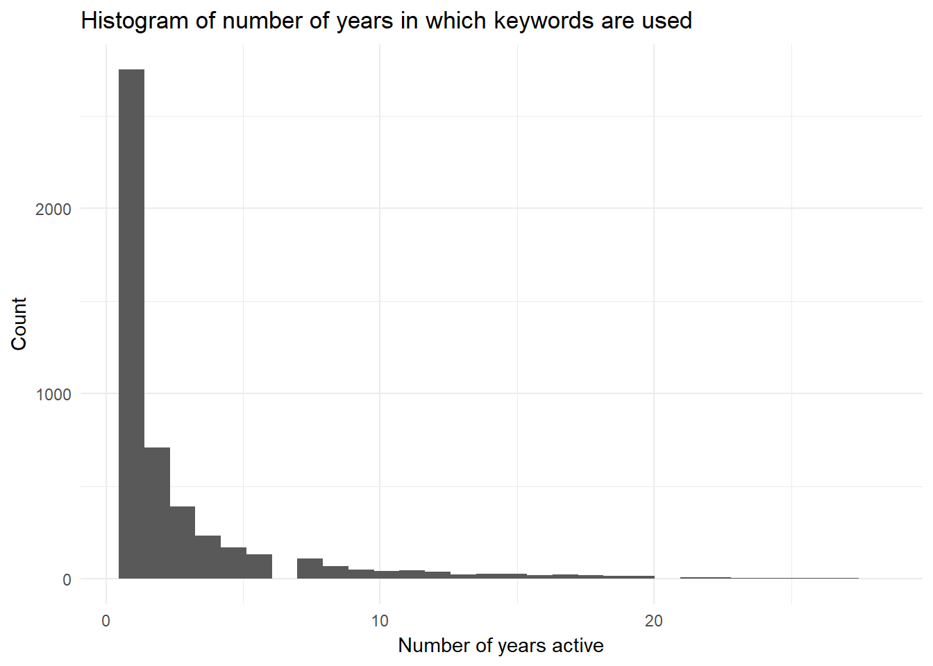
The next variable I am creating is a logical indicator for whether keywords that are cited in more than one year are cited in consecutive years. If they are not cited in more than one year, they have a value of NA; if they are used in more than one year, the value is TRUE when used consecutively and FALSE when there is a gap of more than one year in the use.
keyword.evo$consec <- NA
for (i in 1:nrow(keyword.evo)) {
  year.temp <- test.bind %>%
    filter(keyword == keyword.evo$keyword[i]) %>%
    distinct(year) %>%
    as.matrix() %>%
    diff()

  if (length(year.temp) >= 1) {
    keyword.evo$consec[i] <- all(year.temp == 1)
  } else {
    keyword.evo$consec[i] <- NA
  }

}
summary(keyword.evo$consec)
## Mode FALSE TRUE NA's
## logical 2074 145 2749As the summary shows, only about 3% of keywords are used consecutively, when they are used in more than one year, and the largest plurality of keywords are only used once.
What predicts this pattern?
To begin to look at this, let’s look at the distribution of years for each of the three categories.
keyword.evo.consec.true <- keyword.evo %>%
  filter(consec == TRUE)
consec.true <- test.bind %>%
  filter(keyword  %in% keyword.evo.consec.true$keyword) %>%
  select(-n) %>%
  count(year, sort = TRUE) %>%
  filter(year != 2018) %>%
  mutate(consec = TRUE)

keyword.evo.consec.false <- keyword.evo %>%
  filter(consec == FALSE)
consec.false <- test.bind %>%
  filter(keyword  %in% keyword.evo.consec.false$keyword) %>%
  select(-n) %>%
  count(year, sort = TRUE) %>%
  filter(year != 2018) %>%
  mutate(consec = FALSE)

keyword.evo.consec.na <- keyword.evo %>%
  filter(is.na(consec))
consec.na <- test.bind %>%
  filter(keyword  %in% keyword.evo.consec.na$keyword) %>%
  select(-n) %>%
  count(year, sort = TRUE) %>%
  filter(year != 2018) %>%
  mutate(consec = NA)

consec.evo <- bind_rows(consec.true, consec.false,
                                consec.na)

consec.evo %>%
  ggplot(aes(x = year, y = n, color = consec)) +
  geom_line() +
  xlab("Year") +
  ylab("Keyword count") +
  ggtitle("Trends in keyword usage by consec type")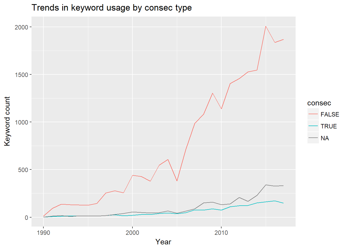
The drastic growth of the FALSE group means that, as time progresses, keywords that are used more than once are being increasingly used inconsistently from year to year. This pattern might indicate recyling.
Before going on, let’s visualize the num.yrs.active by the consec group.
keyword.evo %>%
filter(!is.na(consec)) %>% # NA = one year
ggplot(aes(num.yrs.active, color = consec)) +
geom_density() +
xlab("Number of years a keyword is active") +
ylab("Density") +
ggtitle("Distribution of years active by whether consecutive") +
theme_minimal() 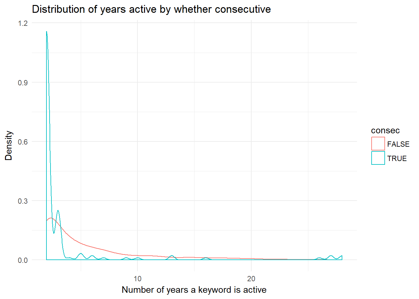 The distibution for each group seems quite different in terms of the keyword “lifespan”. Why?
This point seems like a decent enough cliffhanger at which to stop. The next posts will investigate differences between these three groups of keywords (i.e., single use, inconsistent, and consecutive) and will use structural topic modeling with article abstracts.