
Brandon Sepulvado


In this post, I will be reviewing two principal ways to uncover the topical structure of texts: community detection algorithms on networks of words and topic models. The data I use come from the Web of Science. I have records for all articles containing “bioethic” in their titles, abstracts, or keywords, and the time period ranges from 1900-(Jan.)2018. There are roughly 8,500 articles in this data set (I am happy to provide a much more detailed description upon request).
library(tidytext)
library(readxl)
library(dplyr)
library(stringr)
library(ggplot2)
library(tidyr)
library(igraph)
library(reshape2)
library(tidygraph)
library(stm)In order to run topic models with the article’s abstracts, it is necessary to know k, the number of topics. However, this value is unknown, and there is no non-arbitrary number or range with which to begin. As such, I will start with the number of communities identified from the keyword-keyword network (network), which is a single mode weighted network.
# louvain algorithm
comm_louvain <- cluster_louvain(network)

# label propagation algorithm
comm_label_prop <- cluster_label_prop(network)


#membership(net.comm)
#communities(net.comm)
#crossing(net.comm, network)
#algorithm(net.comm)
#is_hierarchical(net.comm)
#plot(as.dendrogram(net.comm))
The estimates for community number vary quite widely, but, given that only the louvain (63) and label propagation (85) results present a realistic task, I will use the ldatuning package to check fit measures where k varies between 60 and 90. Note: If you would like a detailed comparison of the igraph community detection methods and their relative performances on difference types of networks, I suggest this; the other methods produced wildly divergent estimates for the number of communities (800-3000).
However, before moving further, let’s check out the communities themselves. I first examine the community igraph object obtained with the louvain algorithm. Printing the object gives a preview of the keywords in the first community and indicates that we have 63 groups and a graph modularity of .47. The next function sizes() presents a three-row table; within each row, the top cell indicates the community id and the bottom cell indicates the number of words within it. Finally, return to the short list of the first community members. There obviously seems to be an issue with this method (at least for the first community) because most of the keywords do not intuitively belong together.
# print basic summary
comm_louvain
## IGRAPH clustering multi level, groups: 63, mod: 0.47
## + groups:
## $`1`
## [1] "institutional" "community"
## [3] "personalized" "evidence"
## [5] "review" "based"
## [7] "regenerative" "systematic"
## [9] "precautionary" "emergency"
## [11] "literature" "medicine"
## [13] "principle" "peer"
## [15] "forensic" "alternative"
## [17] "precision" "board"
## + ... omitted several groups/vertices# size of each community
sizes(comm_louvain)## Community sizes
## 1 2 3 4 5 6 7 8 9 10 11 12 13 14 15 16 17 18
## 227 232 207 261 7 3 389 38 6 15 320 458 234 321 4 76 10 3
## 19 20 21 22 23 24 25 26 27 28 29 30 31 32 33 34 35 36
## 16 29 570 14 341 7 2 39 2 2 2 2 2 2 2 2 4 5
## 37 38 39 40 41 42 43 44 45 46 47 48 49 50 51 52 53 54
## 86 4 2 2 2 161 2 5 115 4 150 3 4 2 2 2 6 2
## 55 56 57 58 59 60 61 62 63
## 119 5 2 2 225 2 2 143 2The igraph package makes it easy to visually inspect the sizes of the communities. In the graph using the plot() function, we get a graph in which the x axis lists the communities and the y axis reflects their sizes. This presentation does not easily convey results; the second graph is a histogram. Between the two, it should be relatively easy to see that the vast majority of communities are rather small, but there are a few containing many keywords. I will interpret this finding shortly below, after I get the same information for the other community object.
plot(sizes(comm_louvain))
hist(sizes(comm_louvain))
Let’s replicate the above examination on the label propagation community object. We arrive at 73 communities with this algorithm, but the modularity is drastically lower at .059! We should be skeptical moving forward because there is certainly more conceptual coherence within the bioethics literature. The largest community has 4,609 members, which is problematic: there is likely more nuance within any given subfield of bioethics than that. Further, so many isolated communities with 2-5 members does not correspond to intuitive sense about the field. I will not bother visualizing these results. Do note though that there is at least a bit more coherence in the group of keywords. For example, the words “informed”, “consent”, and “assent” clearly go together, and words, such as “forms” and “psychoses”, relate to the application of this general topic to patient treatment and the process of gaining consent.
# print basic summary
comm_label_prop
## IGRAPH clustering label propagation, groups: 80, mod: 0.04
## + groups:
## $`1`
## [1] "informed" "health"
## [3] "public" "stem"
## [5] "human" "clinical"
## [7] "cell" "palliative"
## [9] "medical" "genetic"
## [11] "organ" "brain"
## [13] "life" "qualitative"
## [15] "advance" "embryonic"
## [17] "assisted" "hiv"
## + ... omitted several groups/vertices# size of each community
sizes(comm_label_prop)## Community sizes
## 1 2 3 4 5 6 7 8 9 10 11 12 13 14 15
## 4602 8 7 9 6 7 4 3 5 2 5 2 2 4 2
## 16 17 18 19 20 21 22 23 24 25 26 27 28 29 30
## 3 2 4 3 2 12 4 8 2 5 8 7 3 3 2
## 31 32 33 34 35 36 37 38 39 40 41 42 43 44 45
## 2 3 4 9 2 6 2 2 2 5 2 12 5 2 6
## 46 47 48 49 50 51 52 53 54 55 56 57 58 59 60
## 2 4 4 4 5 4 6 4 2 3 6 2 2 2 5
## 61 62 63 64 65 66 67 68 69 70 71 72 73 74 75
## 5 5 4 2 3 3 3 3 4 3 2 2 2 2 2
## 76 77 78 79 80
## 2 2 2 2 2At this point, things seem pretty bleak for the community detection algorithms, so we definitely want to check out the topic modeling approaches. However, before we do that, let’s use a different network: one constructed from abstracts instead of keywords. This obviously will change the substantive interpretation of the community structure, but perhaps the keyword network data were simply poorly structured for community detection.1
The following code create a network in which words within abstracts are connected when they appear within the same abstract and have weights which correspond to the number of abstracts in which they co-occur.
abstract_bigrams <- data.bioeth.1 %>%
  filter(!is.na(abstract)) %>%
  unnest_tokens(bigram,
                abstract,
                token = "ngrams",
                n = 2) %>%
  separate(bigram,
           c("word1", "word2"),
           sep = " ") %>%
  filter(!word1 %in% stop_words$word) %>%
  filter(!word2 %in% stop_words$word) %>%
  filter(word1 != "bioethics"
         & word1 != "ethics") %>%
  filter(word2 != "bioethics"
         & word2 != "ethics")

# create weighted edgelist
ab_edges_w <- abstract_bigrams %>%
  count(word1, word2, sort = TRUE)

# create network
ab_network <- ab_edges_w %>%
  rename(weight = n) %>%
  graph_from_data_frame(directed = FALSE)

# verify that edge weights are correct
#setequal(ab_edges_w$n, E(ab_network)$weight)
Now, on to community detection. I will not spend time describing the network here because that is a bit tangential to the purpose of this document.
# louvain algorithm
comm_louvain_ab <- cluster_louvain(ab_network)

# label propagation algorithm
comm_label_prop_ab <- cluster_label_prop(ab_network)
How do the community structures within these objects differ from the previous two? I will begin as before with the community object based upon the louvain algorithm. Now, we have 300 communities with a modularity of 0.38. We can see from the sizes() function that there exists a very large range of community sizes. The first histogram presented illustrates the massive positive skew, and the second histogram, in which I set the maximum x value to 1000, presents the same problem for interpretability. Again, we have a handful of very large topical communities with many tiny communities.
# general info
comm_louvain_ab
## IGRAPH clustering multi level, groups: 300, mod: 0.38
## + groups:
## $`1`
## [1] "stem" "cell"
## [3] "biomedical" "embryonic"
## [5] "research" "empirical"
## [7] "evidence" "semi"
## [9] "scientific" "qualitative"
## [11] "international" "future"
## [13] "depth" "emergency"
## [15] "structured" "based"
## [17] "findings" "community"
## + ... omitted several groups/vertices# community sizes
sizes(comm_louvain_ab)## Community sizes
## 1 2 3 4 5 6 7 8 9 10 11 12 13 14 15
## 2026 3648 1459 1305 1483 1895 1422 3 5 3 3 3 515 17 3
## 16 17 18 19 20 21 22 23 24 25 26 27 28 29 30
## 3 3 5 3 3 6 11 3 3 3 13 3 3 464 2
## 31 32 33 34 35 36 37 38 39 40 41 42 43 44 45
## 3 3 3 3 24 647 3 3 3 2 3 2 2 2 2
## 46 47 48 49 50 51 52 53 54 55 56 57 58 59 60
## 4 2 2 2 2 2 2 2 2 2 34 4 2 2 2
## 61 62 63 64 65 66 67 68 69 70 71 72 73 74 75
## 5 2 2 2 2 2 2 2 2 2 3 2 543 2 2
## 76 77 78 79 80 81 82 83 84 85 86 87 88 89 90
## 2 2 2 2 2 2 2 2 2 2 2 2 2 2 3
## 91 92 93 94 95 96 97 98 99 100 101 102 103 104 105
## 2 2 2 2 2 2 2 5 1142 2 2 64 4 2 2
## 106 107 108 109 110 111 112 113 114 115 116 117 118 119 120
## 2 2 2 2 11 2 3 41 2 2 2 2 2 2 2
## 121 122 123 124 125 126 127 128 129 130 131 132 133 134 135
## 2 2 2 2 2 2 2 2 2 2 2 2 3 4 3
## 136 137 138 139 140 141 142 143 144 145 146 147 148 149 150
## 2 2 2 2 2 1580 2 2 2 2 2 2 320 2 2
## 151 152 153 154 155 156 157 158 159 160 161 162 163 164 165
## 2 2 2 2 2 2 2 2 2 4 2 2325 2 2 2
## 166 167 168 169 170 171 172 173 174 175 176 177 178 179 180
## 2 2 2 2 2 2 2 2 2 2 2 2 2 2 2
## 181 182 183 184 185 186 187 188 189 190 191 192 193 194 195
## 2 2 508 2 2 2 2 2 2 2 2 3 2 2 2
## 196 197 198 199 200 201 202 203 204 205 206 207 208 209 210
## 2 2 2 2 2 2 2 2 2 2 2 2 2 2 2
## 211 212 213 214 215 216 217 218 219 220 221 222 223 224 225
## 2 2 2 2 2 5 2 2 2 2 2 2 2 2 2
## 226 227 228 229 230 231 232 233 234 235 236 237 238 239 240
## 2 2 2 2 2 2 2 2 2 2 2 2 2 4 2
## 241 242 243 244 245 246 247 248 249 250 251 252 253 254 255
## 2 2 1269 2 2 4 2 2 2 2 4 2 2 2 2
## 256 257 258 259 260 261 262 263 264 265 266 267 268 269 270
## 2 2 5 2 2 2 2 2 2 2 2 6 2 3 2
## 271 272 273 274 275 276 277 278 279 280 281 282 283 284 285
## 2 2 2 2 2 2 2 2 2 2 2 2 2 2 2
## 286 287 288 289 290 291 292 293 294 295 296 297 298 299 300
## 2 2 2 2 2 2 2 2 2 2 6 2 2 2 2# plot size distribution
hist(sizes(comm_louvain_ab))
# plot size distribution (truncated x-axis)
hist(sizes(comm_louvain_ab), xlim = c(0, 1000), breaks = 30)
The label propagation gives a slightly larger number of topical communities (416) with an extremely low modularity score of 0.-29. We observed a large modularity difference between the two algorithms in the keyword networks, as well. The largest community contains almost 22,000 members, but there seems to be more variation among the other community sizes. The majority of the remaining communities are not larger than 400 words, so I will truncate the x axis of the following histogram to help (hopefully) with interpretation. It appears that most communities have below 100 members, but there is a non-negligible contingent that contain a few hundred members.
# general info
comm_label_prop_ab
## IGRAPH clustering label propagation, groups: 413, mod: 0.03
## + groups:
## $`1`
## [1] "health"
## [2] "ethical"
## [3] "public"
## [4] "human"
## [5] "stem"
## [6] "bioethical"
## [7] "rights"
## [8] "clinical"
## [9] "cell"
## + ... omitted several groups/vertices# community sizes
sizes(comm_label_prop_ab)## Community sizes
## 1 2 3 4 5 6 7 8 9 10 11 12
## 21841 28 11 6 20 2 3 231 14 6 6 5
## 13 14 15 16 17 18 19 20 21 22 23 24
## 5 4 2 2 4 4 4 11 7 3 26 10
## 25 26 27 28 29 30 31 32 33 34 35 36
## 29 2 6 4 2 2 2 4 14 2 4 6
## 37 38 39 40 41 42 43 44 45 46 47 48
## 2 33 4 15 3 3 3 2 2 2 2 6
## 49 50 51 52 53 54 55 56 57 58 59 60
## 2 2 2 5 2 6 2 13 3 2 2 5
## 61 62 63 64 65 66 67 68 69 70 71 72
## 19 2 2 43 2 3 2 5 2 2 2 2
## 73 74 75 76 77 78 79 80 81 82 83 84
## 3 3 2 2 6 2 5 3 4 2 2 2
## 85 86 87 88 89 90 91 92 93 94 95 96
## 4 3 2 2 2 4 7 3 3 2 8 4
## 97 98 99 100 101 102 103 104 105 106 107 108
## 4 4 3 2 2 2 2 3 4 15 3 3
## 109 110 111 112 113 114 115 116 117 118 119 120
## 4 4 2 2 2 2 3 2 3 2 2 3
## 121 122 123 124 125 126 127 128 129 130 131 132
## 3 2 3 2 2 2 2 10 2 2 2 2
## 133 134 135 136 137 138 139 140 141 142 143 144
## 2 2 2 2 3 2 2 3 2 2 7 2
## 145 146 147 148 149 150 151 152 153 154 155 156
## 2 2 3 7 5 2 2 2 2 3 2 2
## 157 158 159 160 161 162 163 164 165 166 167 168
## 2 4 3 2 2 3 2 5 3 2 2 2
## 169 170 171 172 173 174 175 176 177 178 179 180
## 2 2 2 2 5 4 2 4 3 2 2 3
## 181 182 183 184 185 186 187 188 189 190 191 192
## 2 2 4 2 2 2 2 5 3 2 2 2
## 193 194 195 196 197 198 199 200 201 202 203 204
## 2 4 2 2 2 2 2 7 2 3 2 2
## 205 206 207 208 209 210 211 212 213 214 215 216
## 2 2 2 2 3 4 3 4 2 2 2 2
## 217 218 219 220 221 222 223 224 225 226 227 228
## 2 3 2 2 2 2 2 10 2 2 3 2
## 229 230 231 232 233 234 235 236 237 238 239 240
## 2 2 3 2 2 2 2 3 3 4 3 2
## 241 242 243 244 245 246 247 248 249 250 251 252
## 2 2 2 2 2 2 2 2 2 2 2 2
## 253 254 255 256 257 258 259 260 261 262 263 264
## 4 2 2 2 2 2 2 2 2 2 2 2
## 265 266 267 268 269 270 271 272 273 274 275 276
## 4 2 6 2 2 2 2 3 2 2 2 2
## 277 278 279 280 281 282 283 284 285 286 287 288
## 3 2 2 2 2 2 2 2 2 3 3 2
## 289 290 291 292 293 294 295 296 297 298 299 300
## 2 5 2 3 2 3 2 2 2 2 2 2
## 301 302 303 304 305 306 307 308 309 310 311 312
## 2 2 3 2 2 2 2 2 2 3 2 2
## 313 314 315 316 317 318 319 320 321 322 323 324
## 2 2 1 2 2 2 2 2 2 2 2 6
## 325 326 327 328 329 330 331 332 333 334 335 336
## 2 2 2 2 2 2 3 2 2 2 2 2
## 337 338 339 340 341 342 343 344 345 346 347 348
## 2 2 2 3 2 2 2 2 2 2 2 2
## 349 350 351 352 353 354 355 356 357 358 359 360
## 2 3 2 2 2 2 2 2 2 2 1 2
## 361 362 363 364 365 366 367 368 369 370 371 372
## 3 2 2 2 2 2 2 2 2 2 2 2
## 373 374 375 376 377 378 379 380 381 382 383 384
## 2 2 2 2 2 2 2 2 3 2 2 2
## 385 386 387 388 389 390 391 392 393 394 395 396
## 2 2 2 2 2 2 2 2 2 2 2 3
## 397 398 399 400 401 402 403 404 405 406 407 408
## 1 2 2 2 2 2 2 2 2 2 2 2
## 409 410 411 412 413
## 2 2 2 2 2# plot size distribution
hist(sizes(comm_louvain_ab), xlim = c(0, 400), breaks = 30)
Neither of these two community detection algorithms seems to perform notably well. There are other algorithms one could choose, but, in separate analyses, the others performed still worse. It may very well be the topology of text networks is too distinct and presents computational issues.
Likewise, the problem might rest with this network. One could try further cleaning the data in order to produce a hopeful change in topology, but this change seems doubtful because I have already engaged in a fair amount of cleaning. Thus, for now, we will see how topic models perform.
Topic modeling is an unsupervised form of machine learning: we are asking the function/algorithm to provide us with the topics. We provide a number of documents, the number of topics, and perhaps document-level covariates, and we then receive data on which terms fall within each topic and how the topics vary across documents. This description is of course very crude, and I do not intend this post to constitute an introduction to topic modeling. Rather, I want to compare two methods of arriving at the topical structure of a set of documents.
The key question (at least for me, given my research interests) is precisely the number of topics. Just as community detection can be a difficult and convoluted process for network scientists, identifying k is just as difficult (if not more so at this point in time).
The ldatuning package has a FindTopicsNumber() function that provides a set of diagnostics for models estimated over a set of k values. Let’s use this function to estimate the number of k. We will start with the keyword data (as opposed to the abstract data). Yet, before doing using the FindTopicsNumber() function, I must create a document term matrix. I begin with akw.art.final. Numbers, stop words, bioethics, and ethics have been removed from the akw column. The cast_dtm() function from the tidytext package makes this task very simple.
article_dtm <- akw.art.final %>%
  select(article.id, akw) %>%
  count(article.id, akw, sort = TRUE) %>%
  cast_dtm(article.id, akw, n)
Now, let’s estimate k. I first load the ldatuning package, and then call the function. It requires the document term matrix, the range of topics to be estimated (for which I use 60-90 based upon the community detection results), the metrics from which the performance will be based (I select all available), the Gibbs sampler methods, a seed number for reproducibility, and the number of cores (I use 10 in order to retain two for my normal computing activities while the function is running).
library(ldatuning)

num_k_ftn <- FindTopicsNumber(
  article_dtm,
  topics = seq(from = 60, to = 90, by = 1),
  metrics = c("Griffiths2004",
              "CaoJuan2009",
              "Arun2010",
              "Deveaud2014"),
  method = "Gibbs",
  control = list(seed = 1234),
  mc.cores = 10L,
  verbose = TRUE
)
## fit models... done.
## calculate metrics:
## Griffiths2004... done.
## CaoJuan2009... done.
## Arun2010... done.
## Deveaud2014... done.Now, I want to plot the results. Arun2010 and Deveaud2014 should be minimized, while Grittiths2004 and CaoJuan2009 should be maximized.
FindTopicsNumber_plot(num_k_ftn) The results are far from clear, which is normal when estimating k. I am going to choose 64 because it has roughly the best fit among three of the four metrics. In further versions of these analyses, I will replicate analyses on multiple values of k. Note that regardless of the exact value of k, the number of topics best matches the results from the louvain community detection algorithm.
The above models were estimated using keyword data, which is not particularly desirable because there are so few terms per document. I now want to run models with abstract (that is, the abstracts of the bioethics articles) data. First, I will create a dfm object and then use the quanteda package to convert it into an stm object. This latter step is not absolutely necessary, but it makes easier specifying the components of the stm() function.
# get row == abstract keyword
abstract_words <- data.bioeth.1 %>%
  filter(!is.na(abstract)) %>%
  unnest_tokens(word, abstract) %>%
  anti_join(stop_words,
            by = c("word" = "word")) %>%
  filter(word != "bioethics" &
           word != "ethics") %>%
  filter(!str_detect(word, "\\d")) # remove words containing numbers

# get dfm object to give to stm package
abstract_dfm <- abstract_words %>%
    count(article.id, word, sort = TRUE) %>%
    cast_dfm(article.id, word, n)

# convert to stm object (using quanteda)
library(quanteda)
abstract_stm <- convert(abstract_dfm, to = "stm")
The community detection algorithms provided a starting range for estimating the value of k, but I want to review another option, as well. The stm package has a functionality such that, if you set k equal to zero with spectral initialization, it estimates (a rough starting value for) k, using the algorithm proposed in Lee and Mimno (2014) (see the vignette for further information).
# run stm model to use Lee and Mimno (2014) method
# to estimate k (see vignette p. 13)
searchk_0 <- searchK(documents = abstract_stm$documents,
                     vocab = abstract_stm$vocab,
                     K = 0,
                     init.type = "Spectral",
                     cores = 10)
summary_searchk_0 <- summary(searchk_0)
The code takes longer to run than I want to take each time I compile this file, so I saved the output and will simply load it before calling the stm() function. The searchK() function returned 80 topics as the appropriate starting amount.
stm_0 <- stm(documents = abstract_stm$documents,
             vocab = abstract_stm$vocab,
             K = 80,
             init.type = "Spectral")
## Beginning Spectral Initialization
## Calculating the gram matrix...
## Using only 10000 most frequent terms during initialization...
## Finding anchor words...
## ................................................................................
## Recovering initialization...
## ....................................................................................................
## Initialization complete.
## .....................................................................................................
## Completed E-Step (9 seconds).
## Completed M-Step.
## Completing Iteration 1 (approx. per word bound = -8.120)
## .....................................................................................................
## Completed E-Step (7 seconds).
## Completed M-Step.
## Completing Iteration 2 (approx. per word bound = -7.286, relative change = 1.027e-01)
## .....................................................................................................
## Completed E-Step (7 seconds).
## Completed M-Step.
## Completing Iteration 3 (approx. per word bound = -7.202, relative change = 1.153e-02)
## .....................................................................................................
## Completed E-Step (6 seconds).
## Completed M-Step.
## Completing Iteration 4 (approx. per word bound = -7.180, relative change = 3.053e-03)
## .....................................................................................................
## Completed E-Step (6 seconds).
## Completed M-Step.
## Completing Iteration 5 (approx. per word bound = -7.171, relative change = 1.221e-03)
## Topic 1: studies, research, articles, published, review
## Topic 2: consultation, clinical, community, consultants, research
## Topic 3: paper, based, idea, elements, solidarity
## Topic 4: patient, life, decision, autonomy, patients
## Topic 5: cell, stem, cells, research, ethical
## Topic 6: ethical, issues, principles, dilemmas, practice
## Topic 7: learning, teaching, education, schools, students
## Topic 8: international, research, national, guidelines, ethical
## Topic 9: committee, hospital, care, committees, ethical
## Topic 10: health, public, information, ethical, policy
## Topic 11: life, human, death, care, decisions
## Topic 12: congress, research, panel, medical, world
## Topic 13: bioethical, organ, organs, transplantation, choice
## Topic 14: principle, argument, arguments, autonomy, argue
## Topic 15: countries, developing, health, ethical, global
## Topic 16: risk, competence, cancer, cultural, related
## Topic 17: medicine, practice, health, medical, theological
## Topic 18: research, programs, training, program, academic
## Topic 19: research, children, results, participants, parents
## Topic 20: abortion, health, pregnancy, conscientious, fetal
## Topic 21: historical, article, biology, moral, synthetic
## Topic 22: medicine, author, philosophy, article, queer
## Topic 23: moral, concerns, ethical, public, argue
## Topic 24: medical, medicine, physicians, practice, patients
## Topic 25: embryo, embryos, human, research, ivf
## Topic 26: study, professionals, health, results, care
## Topic 27: genetic, testing, information, ethical, genetics
## Topic 28: consent, informed, patients, research, information
## Topic 29: scientists, issues, social, ethical, bioethicists
## Topic 30: dignity, human, moral, concept, respect
## Topic 31: death, brain, criteria, patients, medical
## Topic 32: animal, animals, welfare, technology, ethical
## Topic 33: empirical, ethical, research, normative, analysis
## Topic 34: ethical, field, science, islamic, neuroethics
## Topic 35: research, issues, commission, bioethical, national
## Topic 36: religious, cultural, religion, ethical, culture
## Topic 37: patients, cancer, study, care, results
## Topic 38: ethical, language, principles, dilemmas, health
## Topic 39: public, research, policy, ethical, science
## Topic 40: research, subjects, ethical, patients, clinical
## Topic 41: human, rights, enhancement, ethical, declaration
## Topic 42: research, participants, consent, clinical, study
## Topic 43: cells, patients, cancer, effects, hl
## Topic 44: trial, hiv, study, trials, placebo
## Topic 45: de, la, research, en, comprehension
## Topic 46: moral, responsibility, change, climate, common
## Topic 47: study, patients, level, ethical, analysis
## Topic 48: health, care, ethical, social, issues
## Topic 49: research, ethical, researchers, clinical, practice
## Topic 50: organ, donation, donors, transplantation, donor
## Topic 51: hope, sex, selection, article, bioethicists
## Topic 52: treatment, decision, decisions, medical, life
## Topic 53: law, legal, genetics, article, genetic
## Topic 54: surgery, ethical, surgical, cosmetic, medical
## Topic 55: clinical, trials, research, drug, patient
## Topic 56: dopamine, myocardial, drug, receptors, effect
## Topic 57: students, education, ethical, study, issues
## Topic 58: rights, research, child, health, pediatric
## Topic 59: vulnerability, research, vulnerable, community, social
## Topic 60: political, social, public, european, democracy
## Topic 61: nursing, human, nurses, global, ethical
## Topic 62: philosophical, social, research, issues, science
## Topic 63: research, scientific, medical, misconduct, science
## Topic 64: patients, physicians, patient, care, ethical
## Topic 65: research, ethical, issues, health, global
## Topic 66: feminist, bioethicists, harm, social, disability
## Topic 67: christian, secular, god, human, moral
## Topic 68: reproductive, assisted, reproduction, art, ethical
## Topic 69: field, moral, theory, medical, clinical
## Topic 70: values, business, medicine, profit, medical
## Topic 71: genomic, laboratory, research, animals, data
## Topic 72: children, parents, blood, study, pediatric
## Topic 73: ethical, medical, patient, clinical, education
## Topic 74: research, human, stem, cell, cloning
## Topic 75: principles, moral, morality, principlism, approach
## Topic 76: ethical, technologies, research, information, genome
## Topic 77: people, ethical, sense, people's, crops
## Topic 78: market, kidney, exploitation, donation, living
## Topic 79: autonomy, human, capacity, social, paper
## Topic 80: medical, health, global, anthropology, cultural
## .....................................................................................................
## Completed E-Step (6 seconds).
## Completed M-Step.
## Completing Iteration 6 (approx. per word bound = -7.168, relative change = 5.281e-04)
## .....................................................................................................
## Completed E-Step (6 seconds).
## Completed M-Step.
## Completing Iteration 7 (approx. per word bound = -7.166, relative change = 2.334e-04)
## .....................................................................................................
## Completed E-Step (6 seconds).
## Completed M-Step.
## Completing Iteration 8 (approx. per word bound = -7.165, relative change = 9.370e-05)
## .....................................................................................................
## Completed E-Step (6 seconds).
## Completed M-Step.
## Completing Iteration 9 (approx. per word bound = -7.165, relative change = 1.422e-05)
## .....................................................................................................
## Completed E-Step (6 seconds).
## Completed M-Step.
## Model ConvergedThere are many diagnostics that should be conducted before settling on a final model. However, the purpose of this exercise is to compare community detection and structural topic modeling methods. So, now that our model has converged, let’s check it out. I display in the following block of code the first three topics.
labelTopics(stm_0, c(1, 2, 3))## Topic 1 Top Words:
## Highest Prob: studies, research, articles, review, literature, published, authors
## FREX: articles, journals, publications, studies, papers, medline, search
## Lift: athletics, coetaneous, coining, cradle, cu, delgado, delgado's
## Score: studies, articles, journals, authorship, publications, papers, medline
## Topic 2 Top Words:
## Highest Prob: consultation, clinical, consultants, community, consultations, care, ethical
## FREX: consultation, consultants, consultations, hecs, competencies, psychiatrists, psychosomatic
## Lift: bxcrrb, hubs, rampart, accredit, accrediting, anticonvulsant, bert
## Score: consultation, consultants, consultations, hecs, competencies, psychiatrists, psychosomatic
## Topic 3 Top Words:
## Highest Prob: paper, based, elements, idea, solidarity, ethical, bioethical
## FREX: introduces, solidarity, elements, idea, ebm, groningen, hospice
## Lift: adduce, admittance, angus, bayertz, biomedicalisation, blasphemous, collage
## Score: solidarity, elements, idea, introduces, ebm, islamic, paperThe four metrics provided for each topic each attempt to capture the relative “importance” of the words (ranked from most to least importance) for each topic. You may refer to the vignette for the stm package to see the equations behind each.
The stm package also has a great plotting function to visualize several aspect of the results. Now, I want to plot the 20 topics that occur with the highest proportion across all documents.
plot.STM(stm_0, type = "summary",
         text.cex = .9, # scale text
         topics = c(1:20), # choose top 20 topics (by proportion)
         n = 4) # list four words for each topic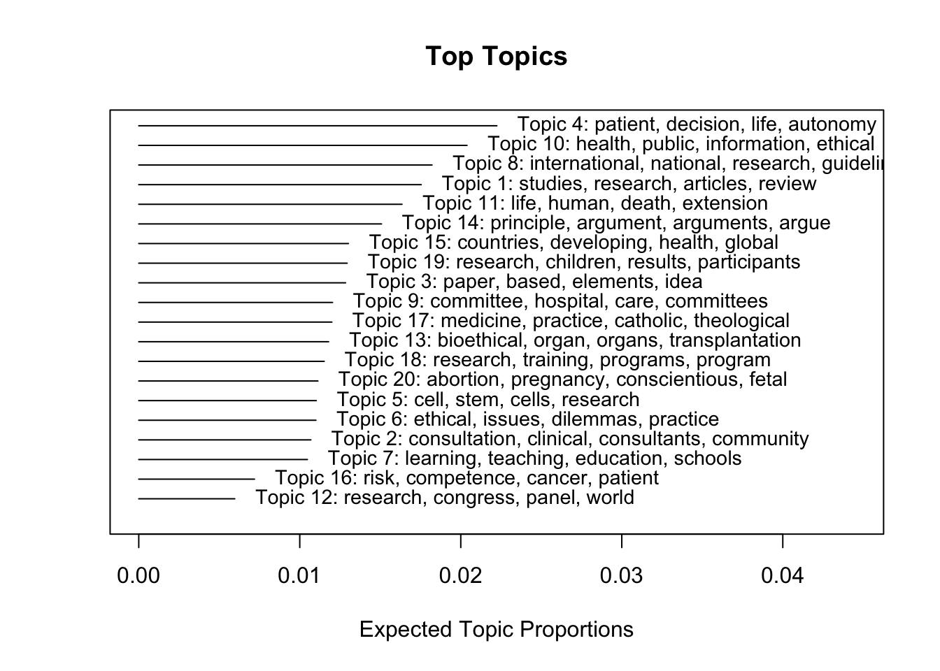
The purpose of this post has been to review the two key ways to identify the topical structure of a set of texts. The community detection methods have performed rather regrettably, but the structural topic models seem to be better. This outcome is good because the stm package makes it easy to use document-level covariates to predict the prevalence of topics. We could now look, for example, at how topics vary over time or by types of authors (e.g., within different countries or disciplines).
One problem however is that with many topics interpretation can be difficult. Emily Erikson (Yale) has proposed a way to inductively arrive at “themes”. Basically, we use the correlation matrix between topics as a weighted network upon which we run community detection algorithms. This approach gives us a relatively small set of themes. We may then more closely interpret trends within and across topics.
As nice as all of this sounds, I will stop here. Addressing these two issues will be the topic of my next post.
A different interpretation would certainly be the case for the following reason. Communities in the keyword network represent sets of institutionalized positions, what one might consider product categories within the bioethical market. Communities in the abstract network will more likely correspond to the topical or conceptual structure of bioethics discourse.↩